就拿TCGA的乳腺癌RNA-seq数据来做个WGCNA示例吧
WGCNA(Weighted Correlation Network analysis)是一个基于基因表达数据,构建基因共表达网络的方法。WGCNA和差异基因分析(DEG)的差异在于DEG主要分析样本和样本之间的差异,而WGCNA主要分析的是基因和基因之间的关系。WGCNA通过分析基因之间的关联关系,将基因区分为多个模块。而最后通过这些模块和样本表型之间的关联性分析,寻找特定表型的分子特征。
网上例子千千万,但是大部分都是从文档翻译而来,要用起来还是有些费劲,要深入的可以移步这里:http://www.stat.wisc.edu/~yandell/statgen/ucla/WGCNA/wgcna.html
下面我将根据TCGA乳腺癌基因表达数据以及乳腺癌压型数据,一步一步的使用WGCNA来进行乳腺癌各个亚型共表达模块的挖掘
#############数据准备#############
首先我们需要下载TCGA 的乳腺癌的RNA-seq数据以及临床病理资料,我这里使用我们自己开发的TCGA简易下载工具进行下载
首先下载RNA-Seq:
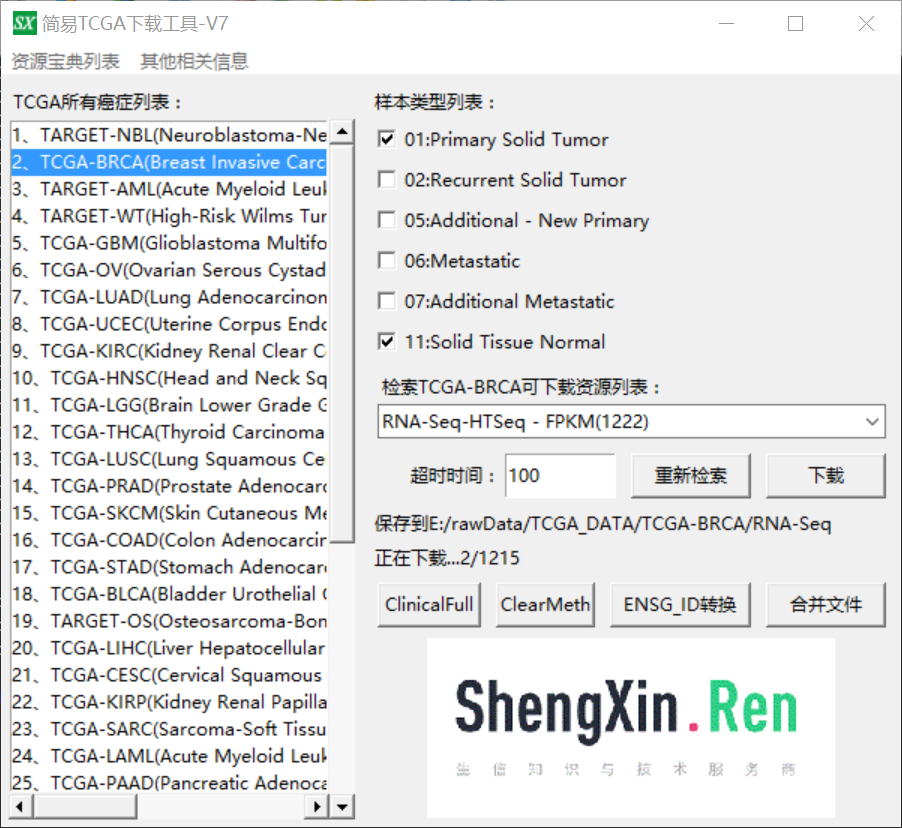
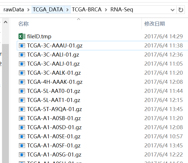
下载之后共得到1215个样本表达数据
进一步下载临床病理资料
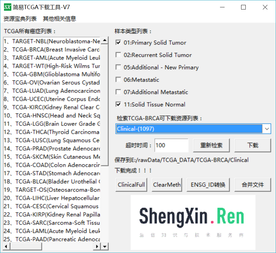
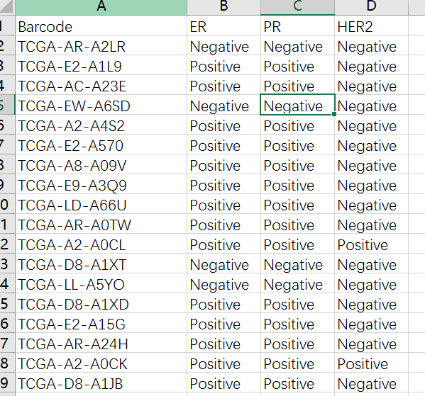
进一步点击 ClinicalFull按钮对病理资料进行提取得到ClinicalFull_matrix.txt文件,使用Excel打开ClinicalFull_matrix.txt文件可以看到共有301列信息,包含了各种用药,随访,预后等等信息,我们这里选择乳腺癌ER、PR、HER2的信息,去除其他用不上的信息,然后选择了其中有明确ER、PR、HER2阳性阴性的样本,随机拿100个做例子吧
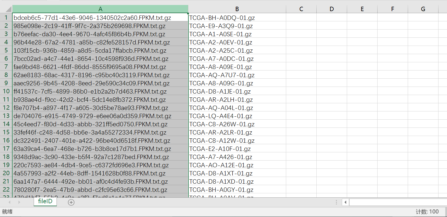
首先打开RNA-Seq数据目录的fileID.tmp(用Excel打开),然后可以看到两列:
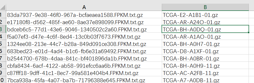
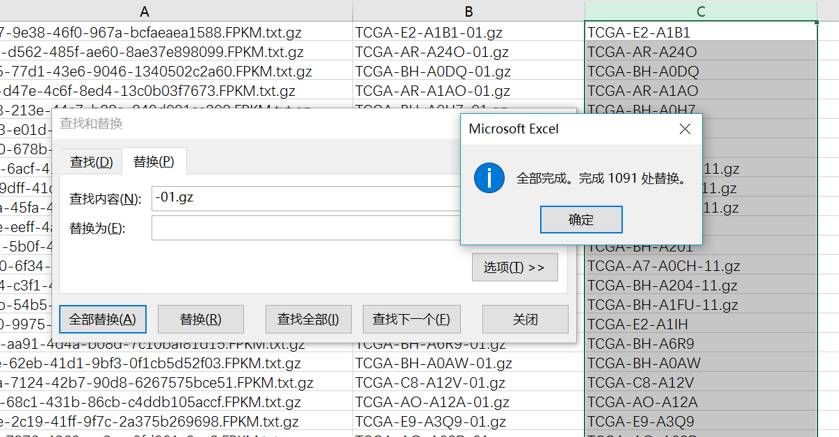
将第二列复制,并且替换-01.gz为空
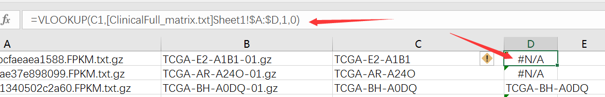
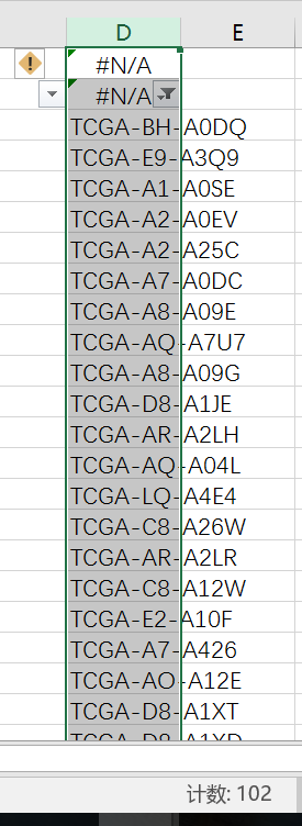
然后筛选非N/A的就得到了这一百个样本对于的RNA-seq数据信息
然后使用TCGA简易小工具“合并文件”按钮就得到表达矩阵了,进一步使用ENSD_ID转换按钮就得到了基因表达矩阵和lncRNA表达矩阵了
#################R代码实现WGCNA##############
setwd('E:/rawData/TCGA_DATA/TCGA-BRCA')
samples=read.csv('ClinicalFull_matrix.txt',sep = '\t',row.names = 1)
dim(samples)
#[1] 100   3
expro=read.csv('Merge_matrix.txt.cv.txt',sep = '\t',row.names = 1)
dim(expro)
#[1] 24991   100
数据读取完成,从上述结果可以看出100个样本,有24991个基因,这么多基因全部用来做WGCNA很显然没有必要,我们只要选择一些具有代表性的基因就够了,这里我们采取的方式是选择在100个样本中方差较大的那些基因(意味着在不同样本中变化较大)
继续命令:
m.vars=apply(expro,1,var)
expro.upper=expro[which(m.vars>quantile(m.vars, probs = seq(0, 1, 0.25))[4]),]##选择方差最大的前25%个基因作为后续WGCNA的输入数据集
通过上述步骤拿到了6248个基因的表达谱作为WGCNA的输入数据集,进一步的我们需要看看样本之间的差异情况
datExpr=as.data.frame(t(expro.upper));
gsg = goodSamplesGenes(datExpr, verbose = 3);
gsg$allOK
sampleTree = hclust(dist(datExpr), method = "average")
plot(sampleTree, main = "Sample clustering to detect outliers"
     , sub="", xlab="")
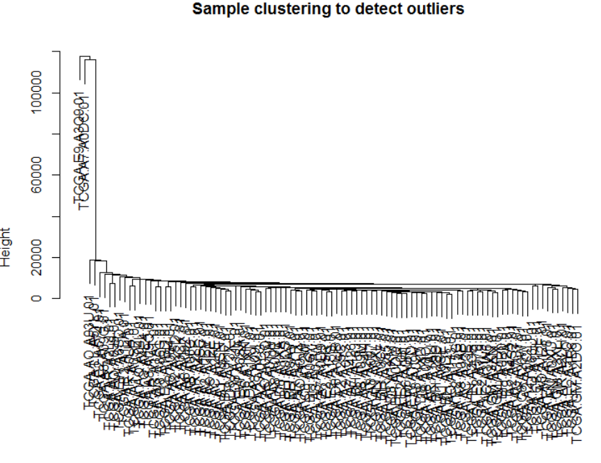
从图中可看出大部分样本表现比较相近,而有两个离群样本,对后续的分析可能造成影响,我们需要将其去掉,共得到98个样本
clust = cutreeStatic(sampleTree, cutHeight = 80000, minSize = 10)
table(clust)
#clust
 #0  1
 #2 98
keepSamples = (clust==1)
datExpr = datExpr[keepSamples, ]
nGenes = ncol(datExpr)
nSamples = nrow(datExpr)
save(datExpr, file = "FPKM-01-dataInput.RData")
得到最终的数据矩阵之后,我们需要确定软阈值,从代码中可以看出pickSoftThreshold很简单,就两个参数,其他默认即可
powers = c(c(1:10), seq(from = 12, to=20, by=2))
sft = pickSoftThreshold(datExpr, powerVector = powers, verbose = 5)
##画图##
par(mfrow = c(1,2));
cex1 = 0.9;
plot(sft$fitIndices[,1], -sign(sft$fitIndices[,3])*sft$fitIndices[,2],
     xlab="Soft Threshold (power)",ylab="Scale Free Topology Model Fit,signed R^2",type="n",
     main = paste("Scale independence"));
text(sft$fitIndices[,1], -sign(sft$fitIndices[,3])*sft$fitIndices[,2],
     labels=powers,cex=cex1,col="red");
abline(h=0.90,col="red")
plot(sft$fitIndices[,1], sft$fitIndices[,5],
     xlab="Soft Threshold (power)",ylab="Mean Connectivity", type="n",
     main = paste("Mean connectivity"))
text(sft$fitIndices[,1], sft$fitIndices[,5], labels=powers, cex=cex1,col="red")
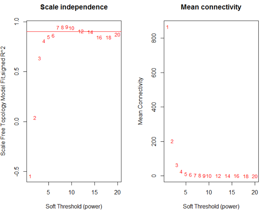
从图中可以看出这个软阈值选择7比较合适,选择软阈值7进行共表达模块挖掘
pow=7
net = blockwiseModules(datExpr, power = pow, maxBlockSize = 7000,
                       TOMType = "unsigned", minModuleSize = 30,
                       reassignThreshold = 0, mergeCutHeight = 0.25,
                       numericLabels = TRUE, pamRespectsDendro = FALSE,
                       saveTOMs = TRUE,
                       saveTOMFileBase = "FPKM-TOM",
                       verbose = 3)
table(net$colors)
# open a graphics window
#sizeGrWindow(12, 9)
# Convert labels to colors for plotting
mergedColors = labels2colors(net$colors)
# Plot the dendrogram and the module colors underneath
plotDendroAndColors(net$dendrograms[[1]], mergedColors[net$blockGenes[[1]]],
                    groupLabels = c("Module colors",
                                    "GS.weight"),
                    dendroLabels = FALSE, hang = 0.03,
                    addGuide = TRUE, guideHang = 0.05)
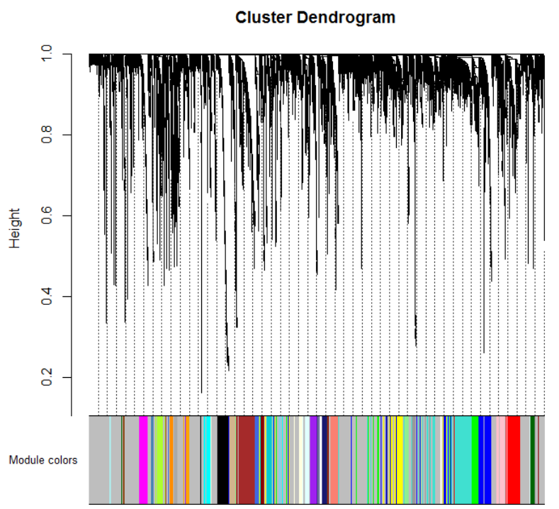
那么做到这一步了基本上共表达模块做完了,每个颜色代表一个共表达模块,统计看看各个模块下的基因个数:

这里就需要咱们利用这些模块搞事情了,举个例子
如果你是整合的数据(整合lnc与gene),那么同时在某个模块中的基因和lncRNA咱们可以认为是 共表达的,这便是lnc-gene共表达关系的获得途径之一了,进一步你可以根据该模块的基因-lnc-基因之间的关系绘制出共表达网络
今天咱们这里不讲这个,而是跟表型关联,咱们已经拿到了这98个样本的ER、PR、HER2阳性阴性信息,那么进一步的咱们可以看看哪些共表达模块跟ER、PR、HER2阴性最相关,代码如下:
moduleLabelsAutomatic = net$colors
moduleColorsAutomatic = labels2colors(moduleLabelsAutomatic)
moduleColorsFemale = moduleColorsAutomatic
MEs0 = moduleEigengenes(datExpr, moduleColorsFemale)$eigengenes
MEsFemale = orderMEs(MEs0)
samples=samples[match(row.names(datExpr),paste0(gsub('-','.',row.names(samples)),'.01')),]#匹配98个样本数据
trainDt=as.matrix(cbind(ifelse(samples[,1]=='Positive',0,1),#将阴性的样本标记为1
      ifelse(samples[,2]=='Positive',0,1),#将阴性的样本标记为1
      ifelse(samples[,3]=='Positive',0,1),#将阴性的样本标记为1
      ifelse(samples[,1]=='Negative'&samples[,2]=='Negative'&samples[,3]=='Negative',1,0))#将三阴性的样本标记为1
)#得到一个表型的0-1矩阵
modTraitCor = cor(MEsFemale, trainDt, use = "p")
colnames(MEsFemale)
modTraitP = corPvalueStudent(modTraitCor, nSamples)
textMatrix = paste(signif(modTraitCor, 2), "\n(", signif(modTraitP, 1), ")", sep = "")
dim(textMatrix) = dim(modTraitCor)
labeledHeatmap(Matrix = modTraitCor, xLabels = colnames(trainDt), yLabels = names(MEsFemale),
               ySymbols = colnames(modlues), colorLabels = FALSE, colors = greenWhiteRed(50),
               textMatrix = textMatrix, setStdMargins = FALSE, cex.text = 0.5, zlim = c(-1,1)
               , main = paste("Module-trait relationships"))
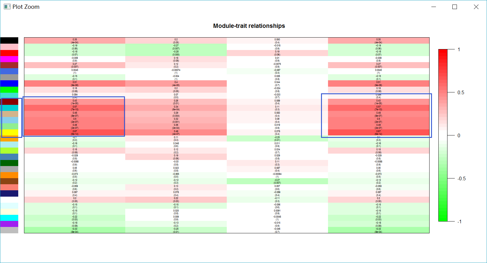 最终找到几个共表达网络与三阴性表型最相关的模块。
modTraitCor = cor(MEsFemale, datExpr, use = "p")
modTraitP = corPvalueStudent(modTraitCor, nSamples)
corYellow=modTraitCor[which(row.names(modTraitCor)=='MEyellow'),]
head(corYellow[order(-corYellow)])
#RAD51AP1     HDAC2     FOXM1    NCAPD2      TPI1      NOP2
#0.9249354 0.9080872 0.8991733 0.8872607 0.8717050 0.8708449
TOM = TOMsimilarityFromExpr(datExpr, power = pow);
probes = names(datExpr)
mc='yellow'
mcInds=which(match(moduleColorsAutomatic, gsub('^ME','',mc))==1)
modProbes=probes[mcInds]
modTOM = TOM[mcInds, mcInds];

dimnames(modTOM) = list(modProbes, modProbes)
cyt = exportNetworkToCytoscape(modTOM,
                                 edgeFile = paste("edges-", mc, ".txt", sep=""),
                                 nodeFile = paste("nodes-", mc, ".txt", sep=""),
                                 weighted = TRUE,
                                 threshold = median(modTOM),
                                 nodeNames = modProbes,
                                 #altNodeNames = modGenes,
                                 nodeAttr = moduleColorsAutomatic[mcInds]);
- 发表于 2017-06-04 10:53
- 阅读 ( 37499 )
- 分类:方案研究