生存分析——R语言
生存分析方法分类
1.参数法:假定生存时间服从某个特定的分布,然后根据分布的特点对生存时间进行分析,常用方法有指数分布法、weibull分步法、对数正态回归分布法等。参数法通过估计的参数得到生存率的估计值,对于两组及多组的样本可根据参数估计对其进行统计推断。
早期应用于武器使用寿命的研究等。
2.非参数法:根据样本的顺序统计量对生存率进行估计,常用的方法有log-rank检验、似然比检验,对于两个及多个生存率的比较,其零假设为两组或多组总体生存时间分布相同,而不对其具体的分布形式及参数进行推断。
常用于随访资料医学研究。
3.半参数法:只规定了影响因素和生存状况间的关系,但是没对时间(和风险函数)的分布情况加以限定。
这种方法主要用于分析生存率的影响因素,属于多因素分析方法,起典型方法是cox比例风险模型。
Cox模型分析法以风险率函数作为应变量,以与生存时间可能有关的协变量或交互项作为自变量来分析生存率。
生存分析使用R包
install.packages("Survival")
library(survival)
survival包中自带数据集ovarian
head(ovarian)
futime fustat age resid.ds rx ecog.ps
1 59 1 72.3315 2 1 1
2 115 1 74.4932 2 1 1
3 156 1 66.4658 2 1 2
4 421 0 53.3644 2 2 1
5 431 1 50.3397 2 1 1
6 448 0 56.4301 1 1 2
其中包含生存时间futime、状态fustat、治疗组别rx、ECOG评分ecog.ps等信息
参数法——survreg()函数
survreg(formula, data, dist, subset)
参数解释:
formula形如Y~X1+X2+X3,但注意生存分析中的应变量Y通常为Surv()函数处理的生存时间;data是数据在R中的名字,subset可以对数据进行筛选。
dist为因变量的分布,包括weibull(weibull分布)、exponential(指数分布)、gaussian(伽马分布)、logistic(logistic分布)、loglogistic(对数logistic分布)和lognormal(对数正态分布)。
示例:
canshufa<-survreg(Surv(futime,fustat)~ecog.ps+rx,ovarian,dist="exponential")
summary(canshufa)
Call:
survreg(formula = Surv(futime, fustat) ~ ecog.ps + rx, data = ovarian,
dist = "exponential")
Value Std. Error z p
(Intercept) 6.962 1.322 5.267 1.39e-07
ecog.ps -0.433 0.587 -0.738 4.61e-01
rx 0.582 0.587 0.991 3.22e-01
Scale fixed at 1
Exponential distribution
Loglik(model)= -97.2 Loglik(intercept only)= -98
Chisq= 1.67 on 2 degrees of freedom, p= 0.43
Number of Newton-Raphson Iterations: 4
n= 26
分析:p=0.43>0.05因此两条生存曲线分布无显著性差异
非参数法——survdiff()函数
survdiff(formula, data, subset, rho)
参数解释:
formula:形如Surv(time, status)~predictors;
data是数据在R中的名字,subset可以对数据进行筛选。
rho数量参数用以指定检验类型,0为log-rank法或Mantel-Haenszel法,1为Wilcoxon法,默认为0。
示例:
survdiff(Surv(futime,fustat)~rx,data=ovarian)
Call:
survdiff(formula = Surv(futime, fustat) ~ rx, data = ovarian)
N Observed Expected (O-E)^2/E (O-E)^2/V
rx=1 13 7 5.23 0.596 1.06
rx=2 13 5 6.77 0.461 1.06
Chisq= 1.1 on 1 degrees of freedom, p= 0.303
分析: p=0.303>0.05,两种治疗方式无显著性差异,所以两种对于卵巢治疗方式没有显著性差异
此外,我们还可以通过绘制其生存曲线来查看结果,所使用的函数为survfit():
示例:
feicanshu<-survfit(Surv(futime,fustat)~rx,data=ovarian)
plot(feicanshu,col=rainbow(2),lty=1,xlab="生存时间/天",ylab="生存率",main="生存曲线")
legend("topright",c("rx=1","rx=2"),lty=1:2,col=rainbow(2))
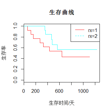 生存曲线呈阶梯状:其中纵坐标为生存率,横坐标为生存时间,线上的短的竖线表示截尾值。
每一级阶梯代表一个死亡时间点(在结尾时间点无阶梯);如果最大时间点是截尾则生存曲线不与曲线相交,否则与横轴相交。
半参数法——coxpy()函数
coxph(formula, data, subset)
参数解释:
formula,形如Y~X1+X2+X3+…+Xn,但Y必须为Surv()函数返回的结果;
data是数据集在R中的名称,subset可以对数据进行筛选
示例:
数据:pcb肝硬化数据
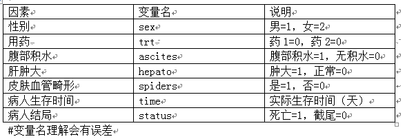
bancanshu<-coxph(Surv(time,status)~sex+trt+ascites+ hepato+spiders,data=mydata)
summary(bancanshu)
Call:
coxph(formula = Surv(time, status) ~ sex + trt + ascites + hepato +
spiders, data = mydata)
n= 292, number of events= 125
(100 observations deleted due to missingness)
coef exp(coef) se(coef) z Pr(>|z|)
sexm 0.35806 1.43056 0.24070 1.488 0.136861
trt 0.05184 1.05321 0.18531 0.280 0.779660
ascites 1.65734 5.24533 0.25286 6.554 5.59e-11 ***
hepato 0.90319 2.46745 0.21273 4.246 2.18e-05 ***
spiders 0.65612 1.92729 0.19702 3.330 0.000868 ***
---
Signif. codes: 0 ‘***’ 0.001 ‘**’ 0.01 ‘*’ 0.05 ‘.’ 0.1 ‘ ’ 1
exp(coef) exp(-coef) lower .95 upper .95
sexm 1.431 0.6990 0.8925 2.293
trt 1.053 0.9495 0.7325 1.514
ascites 5.245 0.1906 3.1955 8.610
hepato 2.467 0.4053 1.6262 3.744
spiders 1.927 0.5189 1.3099 2.836
Concordance= 0.762 (se = 0.028 )
Rsquare= 0.272 (max possible= 0.987 )
Likelihood ratio test= 92.83 on 5 df, p=0
Wald test = 111.7 on 5 df, p=0
Score (logrank) test = 145.8 on 5 df, p=0
分析:给出了风险比对数,风险比,标准误差,p值 ,风险比,置信区间和模型检验等信息
参数检验也基本表明,自变量ascites(腹水积液),hepato(肝肿大),spiders(皮肤血管畸形)对于结果有显著性影响(*表示显著程度)。
基本结果了解后,若要找到最佳模型,我们可以进行变量选择,这里采用逐步回归法进行分析
library(MASS)
bancanshu2<-stepAIC(bancanshu,direction="both")
Start: AIC=1184.05
Surv(time, status) ~ sex + trt + ascites + hepato + spiders
Df AIC
- trt 1 1182.1
<none> 1184.0
- sex 1 1184.1
- spiders 1 1192.8
- hepato 1 1201.0
- ascites 1 1214.8
Step: AIC=1182.13
Surv(time, status) ~ sex + ascites + hepato + spiders
Df AIC
<none> 1182.1
- sex 1 1182.2
+ trt 1 1184.0
- spiders 1 1191.0
- hepato 1 1199.1
- ascites 1 1213.2
由最后结果可以知道,只包含变量ascites,hepato,spiders的模型是最佳模型。
summary(bancanshu2)
Call:
coxph(formula = Surv(time, status) ~ sex + ascites + hepato +
spiders, data = mydata)
n= 292, number of events= 125
(100 observations deleted due to missingness)
coef exp(coef) se(coef) z Pr(>|z|)
sexm 0.3568 1.4288 0.2407 1.483 0.138190
ascites 1.6417 5.1640 0.2465 6.659 2.75e-11 ***
hepato 0.9029 2.4669 0.2127 4.244 2.19e-05 ***
spiders 0.6584 1.9317 0.1970 3.342 0.000831 ***
---
Signif. codes: 0 ‘***’ 0.001 ‘**’ 0.01 ‘*’ 0.05 ‘.’ 0.1 ‘ ’ 1
exp(coef) exp(-coef) lower .95 upper .95
sexm 1.429 0.6999 0.8915 2.290
ascites 5.164 0.1936 3.1852 8.372
hepato 2.467 0.4054 1.6258 3.743
spiders 1.932 0.5177 1.3130 2.842
Concordance= 0.756 (se = 0.027 )
Rsquare= 0.272 (max possible= 0.987 )
Likelihood ratio test= 92.75 on 4 df, p=0
Wald test = 111.9 on 4 df, p=0
Score (logrank) test = 145.8 on 4 df, p=0
绘制生存曲线:
plot(survfit(bancanshu2),col=c("black","darkred","darkgrey"),lty=1,xlab="生存时间/天",ylab="生存率",main="生存曲线")
legend("bottomleft",c("ascites","hepato","spiders"),lty=1:2,col=c("black","darkred","darkgrey"))
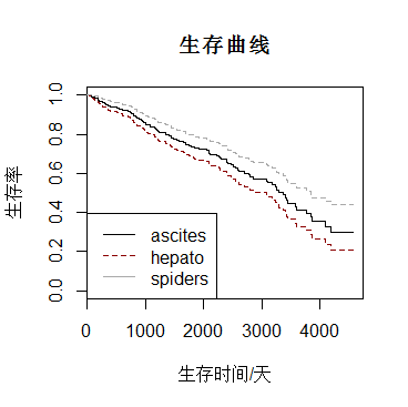
注:数据可能不恰当导致分析有所偏颇
- 发表于 2017-08-18 18:05
- 阅读 ( 24353 )
- 分类:方案研究
